Authored by Samuel Kusangaya*,
Abstract
Different hydro-climatic regions are expected to respond differently to climate change. Despite the availability of downscaled climate data, there is limited knowledge about the skill of downscaled climate data in different hydro-climatic regions of South Africa. Selected catchments included the Buffel’s Catchment in the dry arid region in Northern Cape, Luvuvhu Catchment located in the semi-arid region of Limpopo, uMngeni Catchment in the sub-tropical region of KwaZulu Natal, to the Diep Catchment located within the winter rainfall region of Western Cape. This study is aimed at examining uncertainty in downscaled rainfall and its effect on simulated runoff. The ACRU Model was configured to simulate runoff using the baseline landcover of Acocks JPH [1] veld types. The percentage difference in mean, standard deviation and coefficient of variation metrics were selected for analyzing both rainfall and runoff error propagation. The Indicators of Hydrologic Alteration method was adapted to analyze runoff for each catchment. Results from rainfall analysis showed that GCMs tend to be more uncertain in the estimation of rainfall for catchments in arid areas (Diep and Buffel’s) as compared to catchments in high rainfall areas (uMgeni and Luvuvhu). Results of the annual flow variability showed wider variation in flows for catchments receiving summer rainfall (Luvuvhu and uMngeni), as compared to catchments receiving winter rainfall (Buffels and Diep). It is thus concluded that runoff simulated using GCM climate data is likely to give inconsistent results for both low and high rainfall areas, albeit in different directions: overestimation for low rainfall areas and underestimation for high rainfall areas. The overall conclusion is that, for different hydro-climatic regions, an increase in GCM resolution through more intensive statistical downscaling does not necessarily contribute towards improving the simulation of historical climate data, particularly rainfall. Subsequently, the simulated runoff would also be characterized by uncertainties, not only as inherited / propagated from the input rainfall but also compounded by the different physical catchment characteristics as defined in hydrological modelling.
Introduction
Different hydro-climatic regions are expected to respond differently to climate change. Despite the availability of downscaled climate data, little is currently known about the skill of downscaled climate data in different hydro-climatic regions of South Africa. Given that climate variables such as rainfall are projected to change by varying magnitudes and directions as a result of climate change, it is imperative that we understand the response of different hydro- climatic regions. To this end, the availability of downscaled climate data provides an opportunity for gaining insight into the potential effects of climate change on the hydrology of catchments, in particular those located in southern Africa, one of the most vulnerable regions to climate change [2,3]. Such characterization is particularly critical, given that water resources in southern Africa are already highly variable in space and time and are regarded as a key constraint to the region’s continued socio-economic development [4,5].
To date, a handful of studies carried out in different climatic regions of South Africa, (e.g. [6-8]) have shown evidence of (a) a changing rainfall seasonality for the December - January - February period, which is also the main rainfall season for large parts of southern Africa, (b) a decrease in rainfall during September - October - November period suggesting a reduction in early season rainfall, and (c) a possible decline in the winter rainfall for the western region of South Africa. Furthermore, in the assessment of the implications of climate change for South Africa’s Western Cape Province Midgley GF, et al. [9] found evidence of significant warming trends for particular seasons in the Western Cape. Kruger A [10] reported significant decreases in annual rainfall the northern parts of Limpopo, as well as significant increase0073 in annual rainfall for areas including the northern part of North-West. Both detection studies and climate projections, thus point to changing rainfall patterns, which will consequently result in changing hydrological regimes, since rainfall is the main driver of hydrological systems [11,12]. There is, however, still a dearth in literature on the performance of downscaled climate products, for the current climate. Accordingly, from a hydrological perspective, it is essential that the GCMs are able to realistically reproduce, not only patterns of rainfall Hughes D, et al. [13], but also for the GCM data to produce plausible outputs when used as input to hydrological models.
While there have been several studies on the potential impacts of climate change on southern Africa’s water resources [14-16], there are still considerable uncertainties, not only in current and future climate drivers, but also in terms of how the hydrological systems will respond to climate change [17]. Studies elsewhere [12,18,19] insinuated that the impacts of climat0e change on global and regional water resources are subject to inherent uncertainties, due to data and modelling limitations. Such uncertainties make it difficult to deduce current and future climatological and hydrological implications of climate change. However, the increasing availability of downscaled GCMs climate data such as Coordinated Regional Climate Downscaling Experiment (CORDEX– Africa) Jones C, et al. [20], provide an opportunity for examining these uncertainties [21,22]. More importantly, there is a clear need to examine the uncertainties in downscaled data in different hydro climatic regions at local spatial scales where forcing data is often less accessible but more accurate.
This paper examined the performance of different GCMs, as well as the uncertainty in runoff simulated using downscaled climate data in four diverse hydro-climatic regions of South Africa. Limited studies have been undertaken in southern Africa in this area, despite the availability of downscaled data from the Climate System Analysis Group at the University of Cape Town. The hypothesis that the performance of downscaled GCMs in one hydro climatic region can be used as a basis for using the same in a different region is tested. Knowledge of uncertainties associated with downscaled climate data and consequent simulated runoff aid in increasing our confidence in the use of downscaled climate products in hydrology for future hydrological projections and climate change impact studies.
Materials and Methods
This paper formed part of a larger project aimed at investigating the impact of downscaled input climate data uncertainties on hydrological model outputs. Climate data is made available by climatologists after downscaling, hence from a hydrological perspective it is imperative to first assess the “skill” of the downscaled climate data, particularly in representing rainfall characteristics, before the data were used in runoff simulation. The representativeness of the downscaled GCM rainfall data is evaluated by comparing it with historical rainfall. Thereafter, simulated runoff output generated using historical rainfall was compared to simulated runoff generated using downscaled GCM climate data. Historical daily rainfall data records were extracted from a daily rainfall database for South Africa compiled by Lynch S [23] and only the rainfall stations which had complete data records for the period 1961- 2000 were used in the analysis.
Research Catchments
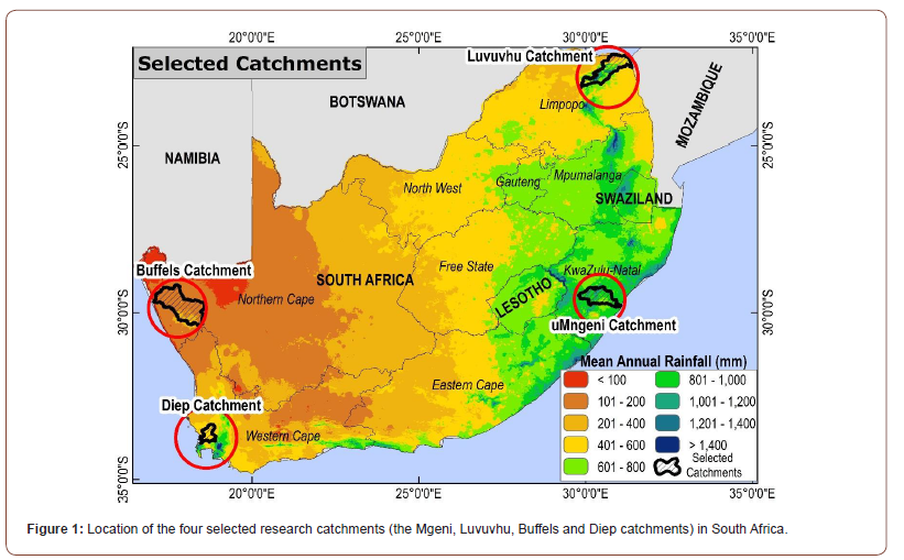
South Africa displays a wide climatic range with mean annual rainfall ranging from < 50 mm to >1400 mm (Figure 1). The rainfall is highly variable both within a year and from one year to the next [24]. This rainfall falls on landscapes varying from steep montane areas to undulating hills to plains. Implying a highly variable spatio- temporal conversion of rainfall to runoff, as well as a regionally and seasonally variable partitioning of the runoff into overland flows, subsurface stormflows, base flows [5].
Four catchments (Figure 1) in different hydro-climatic regions of South Africa were selected, representing diverse climatic conditions. These included the dry arid region in Northern Cape (Buffels Catchment), semi-arid region in Limpopo (Luvuvhu Catchment), sub-tropical region in KwaZulu Natal (uMngeni Catchment) to the winter rainfall region of Western Cape (Diep Catchment). Assessment of hydrological variability was used to analyze runoff data.
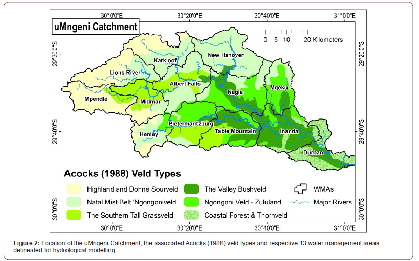
The uMngeni catchment falls within the summer rainfall region in KwaZulu-Natal province of South Africa and generally experiences a warm subtropical climate. The catchment covers around 4 349 km2 and was sub-divided into 13 Water Management Areas (WMAs) (Figure 2). The altitude in the catchment ranges from 1913 m a.s.l in the western escarpment of the catchment to sea level at the catchment’s outlet into the Indian Ocean. The mean annual rainfall (MAP) of the catchment varies from 1 550 mm p.a in the main water source areas in the west of the catchment to 700 mm p.a in the drier middle reaches of the catchment [25]. The rainfall throughout the catchment, is however, highly variable, both interand intra-annually. The mean annual temperature (MAT) ranges from 12°C in the escarpment areas to 20°C towards the coastal areas of the catchment [25].
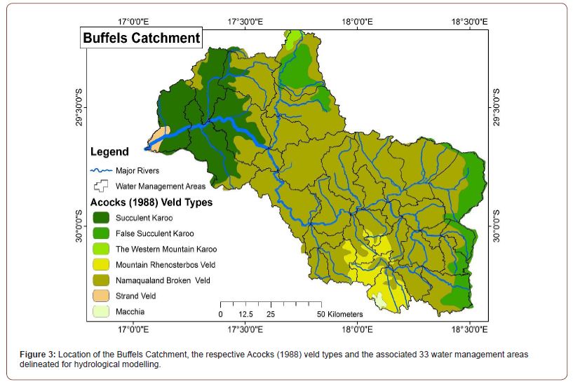
The Buffels catchment falls within the hot and dry Northern Cape Province of South Africa and experiences a semi-arid to arid climate. The Buffels catchment covers around 9 954 km2 and was divided into 33 WMAs for hydrological modelling (Figure 3). The altitude in the catchment ranges from 1579 m a.s.l in the east of the catchment to sea level at the catchment’s outlet into the Atlantic Ocean. The MAP of the catchment varies from 75 mm p.a towards the coast to around 350 mm p.a towards the main source of the Buffels River in the Kamiesberg region [26]. The Buffels River flows during the winter months from May to August, with the Kamieskroon and Springbok regions of the catchment area falling within the winter rainfall zone, whereas the Bushman land peneplain falls within the summer rainfall region [27].
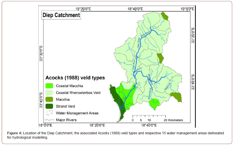
The Diep River catchment is located in the southwestern lowland area of the Western Cape Region in Cape Town (Figure 4). The catchment is low lying and flat with isolated mountains on its eastern boundary and covers a total area of about 1 595 km2. The altitude in the catchment ranges from around 1000 m a.s.l in the north of the catchment to sea level at the catchment’s outlet into the Atlantic Ocean. The Diep River originates from the Riebeek-Kasteel Mountains, north-east of the catchment and flows in a south-westerly direction discharging into Table Bay, north of Cape Town [28]. The Mossel bank River drains the south-eastern portion of the region, in the Durbanville and Kraaifontein areas, and is the main tributary of the Diep River. Climatic conditions in the Diep River catchment are characterized by a winter rainfall regime with high summer evaporation. The catchment experiences frontal precipitation with a MAP varying from around 1200mm in the north-east to 400mm in the south-west [28]. Highest average monthly rainfall occurs between June and August whereas lowest monthly average occurs in December and January with the wettest months occurring from May to October. The mean annual evaporation rate is approximately 1600 mm; hence the river tends to dry up in the summer seasons [28]. Temperature varies from a minimum of 7°C in winter to a maximum of 30 0C in summer [28].
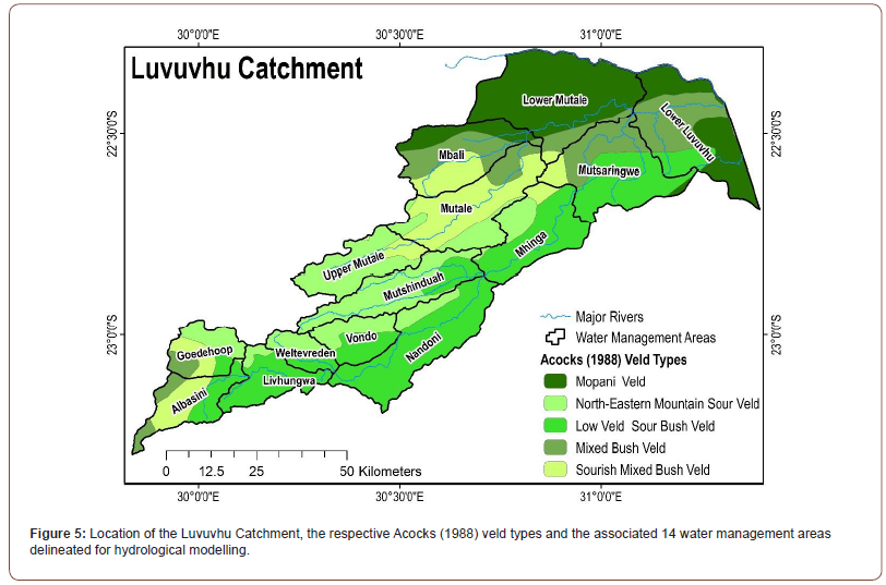
The Luvuvhu Catchment covers around 5 988 km2 and is located in the north-east of the Limpopo Province in South Africa (Figure 5). It is drained by the Luvuvhu and Mutale Rivers, which flow in an easterly direction up to the confluence with the Limpopo River, on the South Africa and Mozambique border. The catchment experiences a dry sub-tropical climate with MATs ranging from 17°C in the mountainous regions to 24°C towards the catchment outlet [29]. The MAP varies from 1870 mm p.a in the mountainous regions (1 360 m.a.s.l) in the upper reaches of the catchment to 300 mm p.a in the drier, lower (200 m.a.s.l) regions of the catchment [29]. The lower reaches of the Luvuvhu catchment fall within the boundaries of Kruger National Park, an important conservation and ecotourism area. The Luvuvhu catchment consists of 14 WMUs (Figure 5) which were delineated according to the Quaternary Catchments and adjusted to accommodate runoff gauging stations.
Downscaled climate data
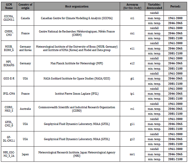
Downscaled climate data was obtained from the Climate System Analysis Group at the University of Cape Town (CSAG – UCT). The climate data were statistically downscaled from the fifth phase of the Coupled Model Inter-comparison Project (CMIP5) at CSAG – UCT using the Self Organizing Map Downscaling (SOMD) method of Hewitson B and Crane R [30]. This set of downscaled climate data have been made readily available to hydrologists for translating climate change signals into impacts on water resources availability. These downscaled climate data were made available in point format and included daily rainfall as well as daily maximum and minimum temperatures. As noted in Hughes D, et al. [13], this data was created from consistent downscaling methods that have been made available for hydrological analyses in South Africa. Table 1 details the characteristics of the downscaled GCM climate data. Rainfall and temperature data from the downscaled climate models were used as input to the ACRU hydrological model and runoff data was simulated.
Table 1: Characteristics of the Downscaled Climate Models obtained from CSAG – UCT which were used in this study.
Hydrological modelling
The ACRU Model was selected for use. It is a physical, conceptual, daily time step process-based model with a multi-soil layer water budget [31]. The ACRU Model was developed in South Africa which means that the parameters are suited for local conditions and the information required to derive parameters is readily available. A principal advantage of using a locally developed model is that its routines are customized to local conditions and locally available data [32]. Generic hydrological data is readily available at a Quaternary Catchment scale for South Africa. Additionally, ACRU has also been used extensively as an aid to decision making in South Africa and beyond. For example, the model has been applied internation ally in hydrological design, the simulation of water resources and research in Botswana, Chile, Germany, Lesotho, Mozambique, Namibia, Swaziland, USA, Canada, and Zimbabwe (e.g., See [33-36]). More details about the ACRU model may be obtained from Schulze R [37] and [31].
The natural vegetation classification system that has been most extensively utilized in South Africa for hydrological modelling purposes is that of Acocks JPH [1] Veld Types, and representative model parameter values exist for all the vegetation types in this system. Using natural land cover variables for hydrological models such as ACRU constitute the datum against which impacts of present land uses on hydrological responses are quantified for water licensing in light of requirements of the South Africa National Water Act (e.g., streamflow reduction activities, or the ecological reserve). Thus, the ACRU Model was configured to use the baseline landcover of Acocks JPH [1] veld types in simulating streamflow for this study.
Values of input variables in the ACRU Model are estimated from the physical characteristics of the catchment (soils, slopes, vegetation, etc.) [31]. Output from the ACRU model can be on a daily basis, or as monthly and annual totals of the daily values of various climate and hydrologically related parameters [38]. The major advantage of such conceptual-physical, non-linear response models is that, because of their high level of process representation and physically based boundary conditions, they can be used with confidence in extrapolations involving “what-if” scenarios of hitherto extreme events or climate variability which may be associated with global change and which are essential ingredients of integrated water resources management [15,39].
For the uMngeni catchment, the configuration of the ACRU model by Warburton M, et al. [29] was adopted in this study. For the Buffels, Luvuvhu and Diep Catchments, configuration of ACRU was modified from the UKZN Centre for Water Resources ACRU configuration of the quinary sub-catchment scale for South Africa Schulze R and Horan M [40], adjusting for the defined WMAs areas, dominant driver (slope and altitude) of hydrological responses within the quinary catchments, as well as the river sub-catchment system derived from the 30m ASTER digital elevation model downloaded from http://www.gdem.aster.ersdac.or.jp/search.jsp. Quaternary catchments are the principal water management units in South Africa and 1946 were demarcated, the quinary catchments are sub delineations of these.
Evaluating downscaled GCM simulations of rainfall for use in hydrological modelling
Runoff response to rainfall is a non-linear process, with a larger proportion of rainfall being converted to runoff when a catchment is wetter, because the soil water antecedent conditions prior to a rainfall event may have been high. Hydrological models are thus particularly sensitive to the rainfall input and any errors in rainfall estimates are amplified in runoff simulations. This implies that the success of hydrological simulation studies depends to a large extent on the accuracy with which either rainfall data are recorded, or rainfall values are generated from climate models such as GCMs [39,41].
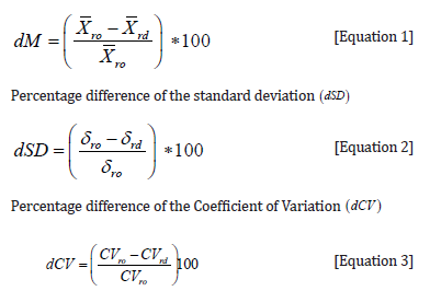
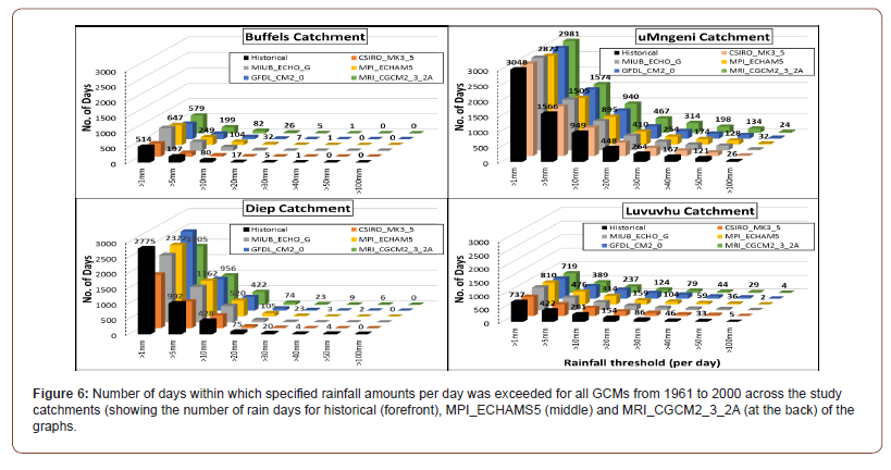
Initially, a frequency analysis of the number of days in which a specified rainfall threshold was exceeded per day was performed for all the rainfall stations at the catchments outlets. A threshold interval of 5mm is used, from rainfall threshold of ≥1 mm to rainfall threshold of ≥100 mm per day. Thereafter, based on a previous study Kusangaya S, et al. [42] (Chapter 4) three metrics were selected as suitable for use in analyzing both rainfall and runoff error propagation, namely percentage difference in mean (dM ) , percentage difference in standard deviation(dSD) , percentage difference of coefficient of variation(dCV ) . These metrics have also been used to quantify uncertainty of modelled climate data in a number of climate studies (e.g., [43-45]). The CV is used to measure the reliability of the multi-datasets mean against the spread of the datasets.
These metrics were considered both “sufficient” and “efficient” measures of error propagation. “Sufficient” in the sense of summarizing all of the relevant information to be gleaned from the rainfall and runoff over sufficiently long periods, and “efficient” in the sense of having the smallest probable error as an estimate of the data long term trends. They are therefore widely used (e.g., [46-49]). Daily rainfall and runoff data were used in the calculations. The dM , dSD and dCV were derived using Equations 1, 2 and 3:
Percentage difference of the mean (dM )
For Equations 1- 3,
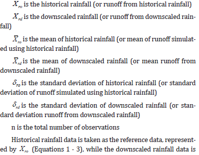
denoted by rd Xrd . Similarly, the simulated runoff simulated using historical rainfall data were denoted by ro X10 and the corresponding simulated runoff from downscaled rainfall is denoted by rd Xrd .
Assessment of hydrological variability
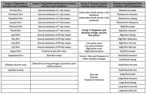
The Indicators of Hydrologic Alteration (IHA) software [50- 52] of the US Nature Conservancy (http://www.nature.org/) was adapted to analyze how downscaled climate data captured and represented runoff in different hydro-climatic regions. The IHA calculates a multi-parameter suite of hydrologic indices representing the major components of the flow regime, and therefore provides a good balance between objective selection of high information indices and accessibility in terms of computation [53]. The full range of IHA multi-variate statistics were used to assess the degree of hydrological alteration between historical and GCM derived hydrological flows. The IHA software calculates a total of 67 parameters, subdivided into two groups - 33 hydrologic alteration parameters and 34 environmental flow component (EFC) parameters [53] (Table 2). The IHA is used in comparing two different flow datasets i.e., simulations from historical climate data vs simulations from GCM climate data. The data record length for analysis is from 1961 to 2000.
Table 2: Summary of hydrological parameters used in the Indicators of Hydrologic Alteration (IHA) and their characteristics (after Richter et al., 1996).
Hydrologic Alteration factor for each of the parameters was calculated after (after [54-56] as follows:
a. For each parameter, IHA divides the full range of ‘pre-impact data’ (i.e., simulations from historical data) into three different categories, generally percentiles (e.g., lowest third, middle third, and highest third).
b. The approach then analyses the ‘post-impact’ (i.e., simulations from GCM data) data and compares the observed distribution of data with the distribution expected from the pre-impact data.
c. Hydrologic Alteration (HA) factor = (observed frequency - expected frequency)/expected frequency.
d. A positive HA factor means that the frequency of values in the category (percentile grouping) has increased in the post-impact period, while a negative HA factor means that the frequency of values in the category (percentile grouping) has decreased in the post-impact period.
Non-parametric (percentile) statistics were used due to the non-normal nature characteristic of hydrologic data. Additionally, the Range of Variability Approach (RVA) described in Richter BD, et al. [50] was implemented. The RVA used the flows simulated using historical climate data as a reference for defining the extent to which “natural flow regimes” differed from flows simulated using GCM data. For the RVA, the runoff data is split into 3 categories: (a) data above 66thpercentile as High RVA, (b) data between 33rdand 66thpercentile as medium RVA, and (c) data below 33rdpercentile as low RVA. Hydrologic Alteration factors, which quantify the degree of alteration of the 33 IHA flow parameters are therefore calculated.
Results
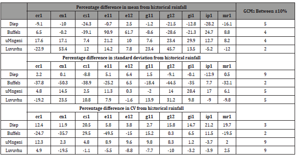
Using the percentage difference of the mean and the percentage difference of standard deviation of GCM from historical rainfall, it was found that there were significant differences in the performance of the different downscaled GCMs in simulating rainfall for the different catchments. Using a threshold of ±10% of historical rainfall mean, 5/10 of downscaled GCMs satisfactorily represented historical rainfall for Diep Catchment, 4/10 for Buffels and uMngeni Catchments, and 2/10 for Luvuvhu Catchment (Table 3). On the other hand, using a threshold of ±10% of historical rainfall standard deviation, 9/10 downscaled GCMs satisfactorily represented historical rainfall for Diep, 2/10 for Buffels Catchment, and 5/10 for uMngeni and Luvuvhu Catchments. Overall, rainfall was better simulated for the Diep, Buffels and the uMngeni catchments whilst it was consistently poorly simulated for the Luvuvhu Catchment.
The four downscaled GCMs which consistently performed well across all the catchments in capturing the mean, standard deviation and CV of historical rainfall were: MIUB ECHO_G (e11) MPI_ ECHAM5 (e12), GFDL_CM2_0 (g11), and MRI_CGCM2_3_2A (mr1). In order to enhance clarity on some subsequent graphs, these GCMs were plotted, even though all the 10 GCMs were used in the analysis.
Table 3: Summary of the percentage difference (of mean, standard deviation, and CV) from historical rainfall for the four catchments. Highlighted (in bold) are the cases where the percentage difference is between ±10% of historical.
Comparison of rainfall thresholds between downscaled GCM and historical rainfall
The nonparametric Wilcoxon Signed Rank Test was used to evaluate if there is a significant difference in the number of days of a given rainfall threshold between historical and GCM rainfall (Table 4). The null (H0) hypotheses that ‘‘there is no significant difference between the number of days of a given rainfall threshold between historical and downscaled modelled rainfall” is assessed using a critical p-value of 0.05. The test is conducted on rain events at rainfall threshold interval of 5 mm (from a threshold of ≥1 mm to ≥100 mm per day).
Table 4: Summary of the nonparametric Wilcoxon Signed Rank Test used to test if there was a significant difference in the number of days of a given rainfall threshold between historical and GCM rainfall (highlighted in bold are the cases where the p-value is < 0.05).
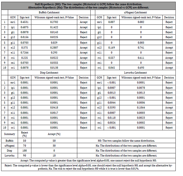
Results showed that for the uMgeni, Luvuvhu and Diep catchments, the distributions of the number of days experiencing a given rainfall threshold (Historical vs GCM) were different resulting in poor estimation of rainfall across all the rainfall thresholds events, and across all the GCMs. For the Buffels Catchment on the other hand, the distribution of the number of days of a given rainfall threshold (Historical vs GCM) largely followed the same pattern, implying that simulation of rainfall is better across most of the GCMs (Table 4 and Figure 6). For all the catchment, however, higher rainfall thresholds of ≥10mm were better estimated when compared to the lower rainfall thresholds across all the GCMs.
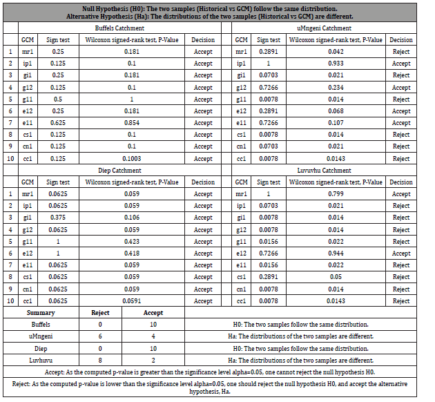
Table 5: Summary of the nonparametric Wilcoxon Signed Rank Test used to test if there is a significant difference in the distribution of the number of days of a given runoff threshold between simulations using historical rainfall vs simulations using GCM rainfall (highlighted in bold are the cases where the p-value is < 0.05).
Comparison of runoff simulated using GCM data and runoff simulated using historical climate data
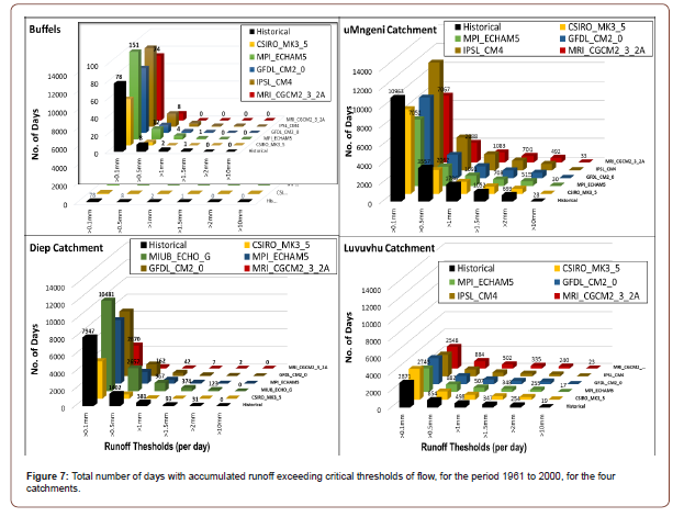
In much the same way that hydrologically critical thresholds of daily rainfall were identified, following the definition of Schulze R [5] five critical thresholds of runoff were used. They are the number of days with:
(a) Flow > 0.1 mm equivalent daily flow, indicating anything above a trickle of (usually) base flow which more than compensates for any evaporative losses from the stream,
(b) Flow ≥ 0.5 mm equivalent daily flow, indicating anything above steady stream flows,
(c) Flow ≥ 1 mm equivalent daily flow, indicating strong flows often from stormflows and thus of relatively short duration,
(d) Flow ≥ 2 mm equivalent daily flow, indicative of quite significant local or regional flooding, and,
(e) Flow ≥ 10mm equivalent daily flow, indicative of extreme local or regional flooding.
Most of the simulated flows using downscaled GCM climate data, were overestimating the number of days runoff exceeded the specified thresholds for the flows simulated using historical climate data (Figure 7). To some extent, catchments with variable rainfall (Luvuvhu and uMngeni) were also characterized by variable total number of days with accumulated runoff exceeding critical thresholds of flow. On the other hand, in catchments where the rainfall is better simulated, runoff is also better simulated across all the GCMs.
The Wilcoxon Signed Rank Test was used to establish if statistically, there is a significant difference in the distribution of the number of days of a given runoff threshold between simulations using historical rainfall vs simulations using GCM rainfall. It was established that for Buffels and Diep, the distribution of the runoff threshold events was comparable, whist for the uMngeni and Luvuvhu catchment, the distribution of the runoff threshold events was not comparable to the events simulated using historical climate data (Table 5).
The overall result for both rainfall and runoff thresholds, is that for Buffels and Diep, both the simulation of rainfall by the GCMs and the subsequent runoff simulations were better across the GCMs albeit with different levels of rejection of the null hypothesis stated. For example, in Buffels catchment, whilst all GCMs agreed in the runoff simulations (that the runoff thresholds were comparable between GCMS and historical), only 50% of the GCMs agreed in the rainfall simulations. Only 30% and 10% of the GCMs simulated rainfall well for the uMngeni and Luvuvhu Catchments respectively. On the other hand, only 40% and 20% of the times were runoff simulated using GCMs comparable to the runoff simulated using historical data for the uMngeni and Luvuvhu Catchments respectively. Overall, there is a vast difference is the skill of the different GCMs in different climatic regions, even though in some of the catchments (Buffels and Diep), rainfall to a greater extent was well simulated.
Error propagation from rainfall to runoff
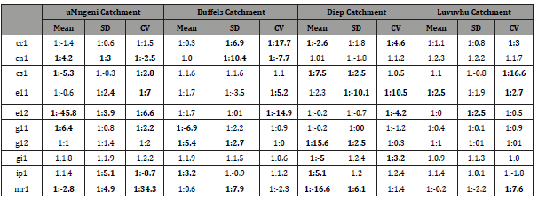
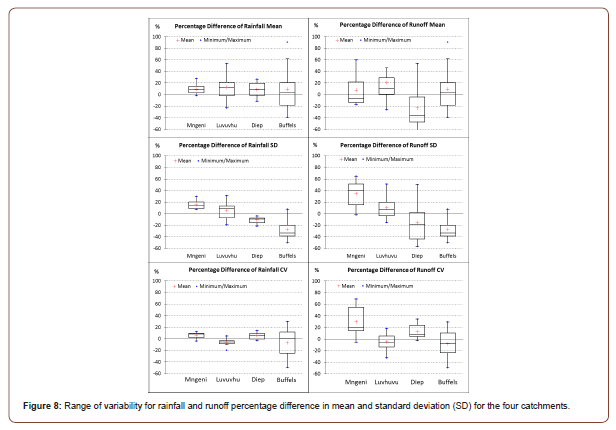
Results of error propagation showed that Luvuvhu and Buffels catchments were characterized by consistently higher percentage differences in the mean and standard deviation of both rainfall and stream flow. This ranged from -15% to 25% for rainfall and -50% to over 25% for stream flow, with extreme percentage differences obtained for runoff of up to 84% error propagation (Figure 8). For the four catchments, the magnitude of error propagation for the mean was higher than for the standard deviation (Table 6). Luvuvhu and uMgeni Catchments were characterized by higher error propagation ratios than Diep and Buffels catchments. Furthermore, Buffels, Diep and Luvuvhu catchments had at least four GCMs showing error propagation greater than 1:2 for the coefficient of variation as compared to seven GCMs for the uMngeni Catchment. Overall, the uMngeni Catchment had the highest error propagation ratios in all the metrics used as compared to the other three catchments.
Table 6: Error propagation ratios of the mean, standard deviation (SD) and coefficient of variation (CV) for the four catchments, highlighting (in bold) where the error propagation ratios are greater than 1:2 from rainfall to runoff for the respective GCMs.
Magnitude and duration of annual extreme flows
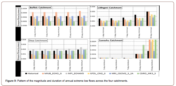
A suit of indices depicting magnitude and duration of annual extreme runoff conditions (low and high flows indices) were calculated in the Parameter Group 2 of the IHA. These included the 1-, 3-, 7-, 30-, and 90-day minimums and maximums taken from moving averages calculated (as means) for every period that is completely within the water year (October – September) [52]. The magnitude of low flows showed marked differences from catchment to catchment and for the different thresholds. The uMngeni, Buffels and Diep Catchments did not show extreme fluctuations for the within catchment magnitude of low flows for both the historical and the GCM simulated stream flows. However, Luvuvhu catchment showed marked differences in magnitude of low flows across all thresholds, with massive over simulation of the 90 day minimum from the downscaled GCM climate data. MIUB_ECHO_G (e11), MRI_CGCM2_ 3_2A (mr1) and MPI_ECHAM5 (e12) captured well the pattern of 1-, 3-, 7-, 30-, and 90-day minimums for the uMngeni, Diep and Buffels Catchments. The duration was found to have a consistent pattern across all GCMs and across the indices thresholds (1 to 90 days minimums), except for Luvuvhu Catchment (Figure 9). The uMngeni Catchment, however, showed a gradually increasing magnitude with increasing duration with the 90 day minimum having the corresponding highest magnitude. Overall, low flow indices were under simulated in some catchments (e.g., uMngeni) and overstimulated in others (e.g., Buffels).
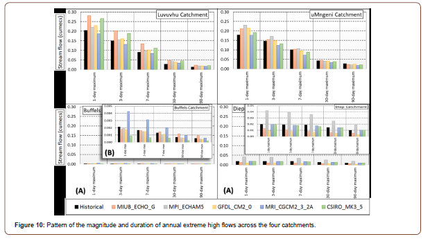
High flows also exhibited marked differences both in terms of magnitude and duration from catchment to catchment and from the different indices thresholds, but there is consistent over simulation of the high flows for all the threshold levels across all catchments (Figure 10). GCM MRI_CGCM2_3_2A (mr1) under simulated extreme high flows in Luvuvhu and uMngeni catchments. On the other hand, GCM MIUB_ECHO_G (e11) over simulated in Luvuvhu and uMngeni catchments.
Range of runoff variability for the four catchments
The range of variability analysis (RVA) used the pre-development (here taken as runoff simulation from historical climate data) natural variation of IHA parameter values as a reference for defining the extent to which natural flow regimes are altered when using downscaled GCM climate data to drive the models (see [50,55,56]). The maximum HA value is infinity, with a minimum value of -1. As mentioned earlier, a positive HA value implies that the frequency of values in the category (high, medium, and low RVA) is higher for the runoff simulated using the historical climate data (pre-impact) as compared to runoff simulated using the GCM climate data (post impact). A negative value means that the frequency of values in the category is lower for the runoff simulated using the historical climate data as compared to runoff simulated using the GCM climate data.
Runoff data was split into 3 categories: (a) data above 66th percentile - high RVA, (b) data between 33rd and 66th percentilemedium RVA, and (c) data below 33rd percentile - low RVA. Overall, results from the four catchments showed that in the high and middle RVA ranges, all GCMs in all months of the year showed negative values indicating that runoff simulated from historical climate data was less than runoff simulated from GCMs climate data (overestimation). On the low RVA category, however, the uMngeni, Buffels and Diep Catchments showed positive HA than the Luvuvhu catchment (Figure 11 & 12).
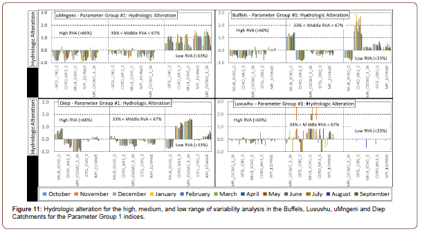
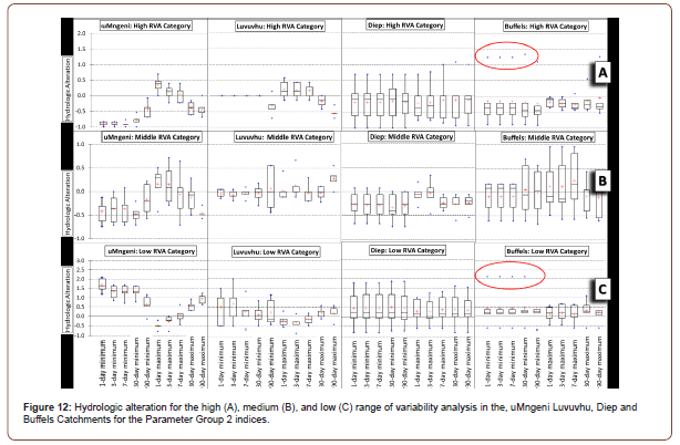
Summary of hydrologic alteration for the Parameter Group 2 indices for low flows and high flows analysis is shown in Figure 12. For the medium and high RVA (Figure 12 A & B), for all catchments, the HA is largely negative showing that the frequency of values in the medium and high RVA category was lower for the runoff simulated using the historical climate data as compared to runoff simulated using the GCM climate data. The uMngeni and Luvuvhu catchments, however, had some indices (1-, 3-, and 7 day maximum) with HA greater than 1. These two catchments also receive the highest amount of rainfall and consequently have higher maximum flows. Buffels catchment on the other hand was characterized by some extreme values in the high RVA category and this indicated the influence of occasional high rainfall resulting in the extremes in the (1-, 3-, 7-, 30-, and 90 day minimum flows (Figure 12a). The low RVA category was characterized by positive HA for the catchments, except for Luvuvhu which had some indices (1-, 3-, and 7 day maximum) with low HA. This implied that that the frequency of values in the low RVA category was higher for the runoff simulated using the historical climate data as compared to runoff simulated using the GCM climate data.
Discussion and Conclusions
This paper examined uncertainty in rainfall and runoff from downscaled climate data in diverse hydro-climatic regions of South Africa. The selected catchments varied from the Buffels Catchment in the dry arid region in Northern Cape, Luvuvhu Catchment located in the semi-arid region of Limpopo, uMngeni Catchment in the sub-tropical region of KwaZulu Natal, and the Diep Catchment located within the winter rainfall region of Western Cape. Analysis of rainfall showed that for the Diep, Luvuvhu and uMngeni Catchments there was a poor estimation of rainfall across all the rainfall thresholds events, and across most GCMs. For the Buffels catchment, however, the simulation of rainfall by the GCMs was good across all the rainfall thresholds and across most GCMs. Using the runoff threshold events, it was established that for Buffels and Diep Catchments, the distribution of runoff threshold events was comparable, whist for the uMngeni and Luvuvhu Catchments, the distribution of the runoff threshold events was not comparable to the events simulated using historical climate data.
The overall result for both rainfall and runoff thresholds analysis, showed that for Buffels catchments, both the simulation of rainfall events by the GCMs and the subsequent runoff events simulations were better across the GCMs, albeit with different levels of skill for the different GCMs. The skill of the GCMs in simulating the mean, standard deviation, and coefficient of variation, was however, inconsistent with the results from the rainfall and runoff thresholds analysis. Buffels and Luvuvhu catchments were simulated marginally well (6/10 GCMs) for the percentage difference in mean, even though the variability was not well captured. For Diep and uMngeni catchments, however, both the mean and SD were poorly simulated. Additionally, analysis of simulated runoff showed that catchments receiving low (Luvuvhu) to exceptionally low (Buffels) rainfall were characterized by high inter GCM variability in simulated runoff as compared to catchments in moderately high (Diep) to high (uMngeni) rainfall. Thus, the conclusion from the threshold events analysis is that GCMs tend to be more certain in the estimation of both rainfall and runoff events for catchments in arid areas as compared to catchments in high rainfall areas. When considering both analysis of threshold events and percentage differences, the skill of the different GCMs in different climatic regions varied widely and therefore it is recommended that for climate impact analysis, the skill of the different GCMs have to be evaluated before use.
In moderately high to high rainfall catchments, runoff simulated using GCMs underestimated runoff simulated using historical climate data. On the other hand, in semi-arid and arid catchments runoff simulated using GCMs overestimated runoff simulated using historical climate data. Thus, it is concluded that runoff simulated using GCM climate data is likely to give uncertain simulation results for both low and high rainfall areas, albeit in different directions: overestimation for low rainfall areas and underestimation for high rainfall areas.
Catchments receiving summer rainfall were characterized by wider variation in flows as compared to catchments receiving winter rainfall. This could be explained by the mechanisms causing the rainfall. It is widely reported in literature, for example [2,5,57,58] that GCMs are less capable of simulating second order atmospheric processes, such as rainfall, compared to first order atmospheric processes, such as surface heat and vapor fluxes. This, in turn results in the following limitations as outlined by Schulze R [5]: (a) failure to simulate individual convective rainfall events, which poses problems in many parts of the world, including most of southern Africa, where convective rainfall is a dominant form of rainfall; (b) difficulty in simulating the intensity, frequency and distribution of extreme rainfall; and, (c) simulating too many light rainfall events (< 2 mm.day-1) and generally too few heavy rainfall events (> 10 mm.day-1), whilst maintaining a fairly realistic mean rainfall. Combined, these factors tend to reduce the accuracy of rainfall from GCMs and the subsequent simulated streamflow, as was noted in this study.
When runoff data was split into percentiles, median flows for all the runoff data above 67th percentile and data between 33rd and 66th percentile showed that the runoff simulated from historical climate data was less than runoff simulated from GCMs climate data. This implied that runoff data from GCMs overestimated runoff simulated from historical climate data for moderately high to high flows. On the other hand, for the data below the 33rd percentile, positive HA implied that the frequency of values in the low HA category was higher for the runoff simulated using the historical climate data (pre-impact) as compared to runoff simulated using the GCM climate data (post impact). Thus, it meant that low flows were mostly underestimated by runoff simulated using GCMs as compared to runoff simulated using historical data. Again, these observations in simulated stream flows can be attributed to the limitations observed, in generated downscaled GCM data, vis-à-vis, the inability of GCMs to simulate second order atmospheric processes as outlined in Giorgi F, et al. [57] and Solomon S, et al. [2].
Even though some of the downscaled climate data utilized in this study had shown elsewhere [42,59] that it had the least variability and simulated historical rainfall satisfactorily, the results of this analysis showed that even with a satisfactory simulation of rainfall in one catchment area, GCMs still retain significant model uncertainty especially when applied to different hydro climatic regions. Furthermore, it is evident that not only do climate models produce different responses to the same greenhouse gas forcing due to varying dynamics and physics parameterizations (“model configuration” uncertainty), but also the different initial conditions can produce different responses to the same greenhouse gas forcing because of nonlinearities within the climate system (“internal variability” uncertainty) [45,57,58,60,61]. Therefore, it is primarily a result of limitations of the climate model structure and parameterization used to represent geophysical processes [8,61] that explains most of the uncertainty.
Additionally, whilst downscaling produces climatic information at scales finer than the initial projections, it involves using additional information, data, and assumptions, which leads to further uncertainties and limitations of the results (see, e.g., [20,62-65]). Accordingly, the fact that climate models perform well in one region should not be used as a precondition of their use in a different region. As shown in this study, downscaled GCMs are prone to producing different results depending on the hydro-climatic conditions of the different regions. Thus, the ability of the downscaled GCMs to “skillfully” represent historical rainfall, that which is the main driver in hydrological modelling, is affected by the regional hydro climatic characteristics.
Additionally, whilst downscaling produces climatic information at scales finer than the initial projections, it involves using additional information, data, and assumptions, which leads to further uncertainties and limitations of the results (see, e.g., [20,62-65]). Accordingly, the fact that climate models perform well in one region should not be used as a precondition of their use in a different region. As shown in this study, downscaled GCMs are prone to producing different results depending on the hydro-climatic conditions of the different regions. Thus, the ability of the downscaled GCMs to “skillfully” represent historical rainfall, that which is the main driver in hydrological modelling, is affected by the regional hydro climatic characteristics.
To read more about this article...Open access Journal of Hydrology & Meteorology
Please follow the URL to access more information about this article
To know more about our Journals...Iris Publishers
To know about Open Access Publishers


No comments:
Post a Comment